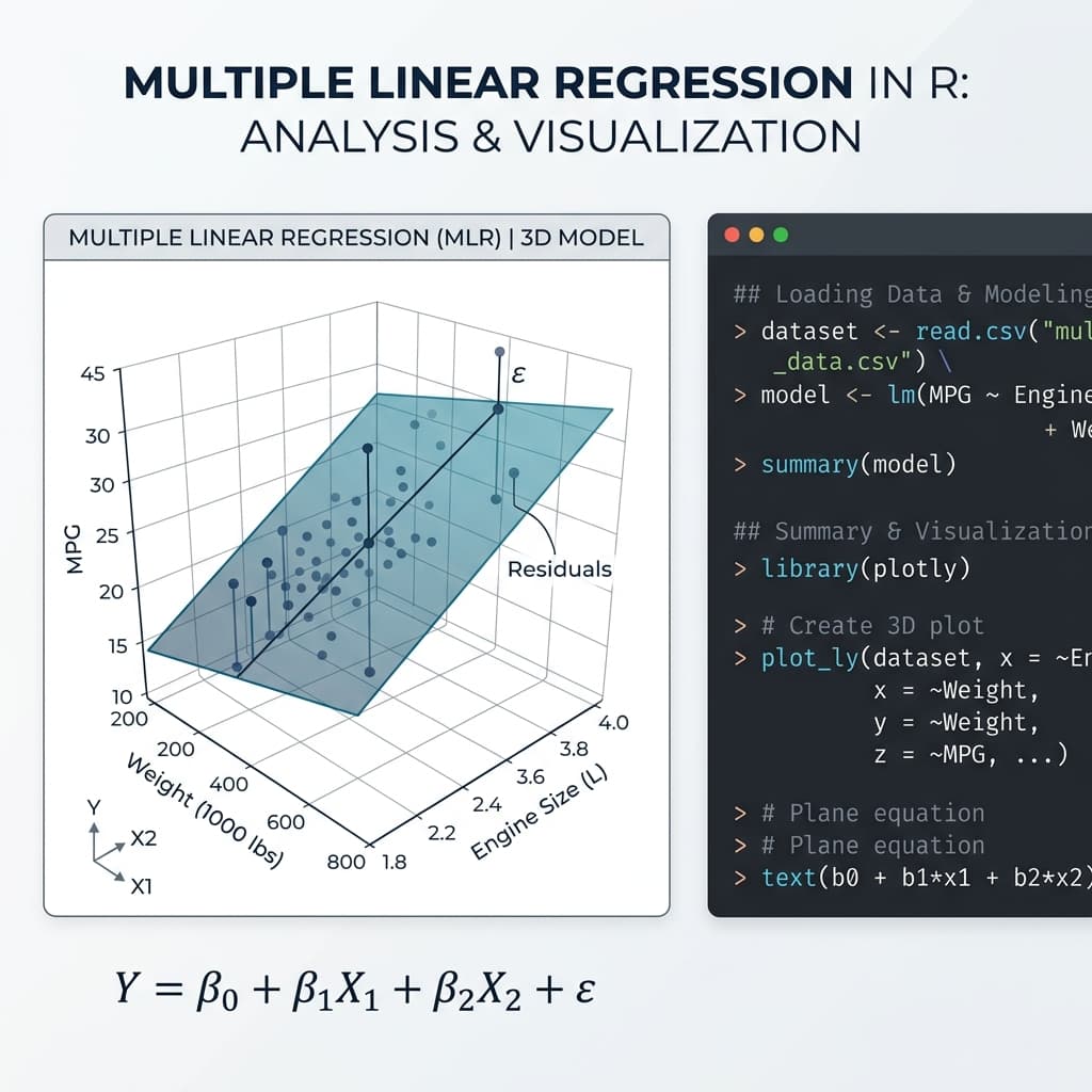
Multiple Linear Regression (MLR) is a foundational statistical technique used to model the relationship between a single continuous dependent variable and two or more independent variables. In academic research, data science, and business analytics, mastering multiple regression enables you to control for confounding factors, isolate the effect of specific predictors, and make robust predictions. R, being a statistical powerhouse, offers an exceptionally intuitive and comprehensive environment for performing regression analysis, evaluating assumptions, and visualizing results.

This comprehensive guide will walk you through the entire process of conducting a multiple linear regression in R. We will cover data preparation, building the model using the lm() function, verifying statistical assumptions through diagnostic plots, and, most importantly, interpreting the output with the nuance expected in rigorous academic research. Whether you are transitioning from point-and-click software (see our comparison of R vs SPSS for dissertation work) or solidifying your statistical foundation, this guide will provide the depth you need.

1. Understanding the Multiple Regression Model

Before diving into the code, it is crucial to understand the mathematical framework underlying multiple regression. The model assumes a linear relationship between the dependent variable (Y) and the independent variables (X₁, X₂, ..., Xₖ). The population model is expressed as:

Y = β₀ + β₁X₁ + β₂X₂ + ... + βₖXₖ + ε

• Y (Dependent Variable): The outcome you are trying to predict or explain. It must be continuous (interval or ratio scale). If your dependent variable is categorical, you should consider logistic regression instead. (Unsure which test to use? Consult our Statistical Test Decision Tree).
• X₁, X₂, ..., Xₖ (Independent Variables): The predictors. They can be continuous or categorical (represented as dummy variables).
• β₀ (Intercept): The expected value of Y when all independent variables are exactly zero.
• β₁, β₂, ..., βₖ (Coefficients): The partial regression coefficients. β₁ represents the expected change in Y for a one-unit increase in X₁, holding all other variables in the model constant. This ceteris paribus assumption is the core advantage of MLR.
• ε (Error Term/Residual): The difference between the observed value and the value predicted by the model. Regression minimizes the sum of squared residuals (Ordinary Least Squares or OLS).

2. Data Preparation and Exploration in R

Let's simulate a dataset commonly encountered in social science or educational research. We will predict a student's final university grade (Final_Grade, scale 0-100) based on their Study_Hours per week, their Previous_Score (scale 0-100), and their Attendance rate (percentage).

# Set seed for reproducibility
set.seed(123)

# Generate synthetic dataset
n <- 200
Study_Hours <- rnorm(n, mean = 15, sd = 5)
Previous_Score <- rnorm(n, mean = 70, sd = 10)
Attendance <- rnorm(n, mean = 85, sd = 8)

# Generate dependent variable with some random noise (error term)
# Formula: Grade = 10 + 1.5*(Study) + 0.5*(Prev) + 0.3*(Att) + error
Error <- rnorm(n, mean = 0, sd = 5)
Final_Grade <- 10 + (1.5 * Study_Hours) + (0.5 * Previous_Score) + (0.3 * Attendance) + Error

# Constrain grades to a maximum of 100
Final_Grade[Final_Grade > 100] <- 100

# Create dataframe
student_data <- data.frame(Final_Grade, Study_Hours, Previous_Score, Attendance)

# View first few rows
head(student_data)

Before running the regression, it is standard practice to examine the descriptive statistics and bivariate correlations to ensure there are no glaring data entry errors and to get a preliminary sense of the relationships.

# Summary statistics
summary(student_data)

# Correlation matrix
cor(student_data)

3. Building the Multiple Regression Model

In R, the workhorse for linear modeling is the lm() function. The syntax requires a formula specifying the dependent variable followed by a tilde (~), and then the independent variables separated by plus signs (+). Finally, you specify the data frame.

# Fit the multiple linear regression model
model_1 <- lm(Final_Grade ~ Study_Hours + Previous_Score + Attendance, data = student_data)

# Display the summary of the model
summary(model_1)

4. Deep Dive: Interpreting the Regression Output

When you run summary(model_1), R produces a dense block of text. For beginners, this can be overwhelming. Let's break it down section by section, providing the statistical nuance required for academic reporting.

4.1 Residuals

The first section of the output summarizes the residuals (the differences between observed and predicted values). You want the median to be close to zero, and the min/max and 1Q/3Q values to be roughly symmetrical. Extreme asymmetry might suggest outliers or a non-normal error distribution, which we will test formally later.

4.2 Coefficients

This table is the heart of your analysis. It contains the estimates for your intercept and slopes.

• Estimate (β): This column provides the unstandardized coefficients.
  • Intercept: The predicted Final_Grade if Study Hours, Previous Score, and Attendance were all exactly zero. In many contexts, an intercept doesn't have a practical, real-world meaning (e.g., it's impossible to have 0% attendance and a 0 previous score while still enrolled), but it anchors the regression plane.
  • Study_Hours: For every one additional hour of study per week, a student's Final Grade is predicted to increase by the coefficient amount, holding Previous Score and Attendance constant.
• Std. Error: This represents the average distance that the observed values fall from the regression line. More importantly, it measures the precision of the coefficient estimate. A smaller standard error indicates a more precise estimate. It is used to calculate the t-statistic.
• t value: Calculated as the Estimate divided by its Standard Error (Estimate / Std. Error). It measures how many standard deviations our coefficient estimate is away from zero. Larger absolute t-values provide stronger evidence against the null hypothesis (that the true coefficient is zero).
• Pr(>|t|) (p-value): This is the probability of observing a t-value as extreme or more extreme than the one calculated, assuming the null hypothesis is true. Crucial Note: A p-value less than your chosen alpha level (usually 0.05) does not "prove" your hypothesis, nor does it measure the size or importance of the effect. It simply indicates that the observed relationship is unlikely to have occurred by chance under the null hypothesis model. Do not conflate statistical significance with practical significance.

4.3 Model Fit: R-squared and Adjusted R-squared

At the bottom of the summary, R reports metrics evaluating how well the overall model fits the data.

• Multiple R-squared (R²): The proportion of the variance in the dependent variable that is predictable from the independent variables. An R² of 0.65 means that 65% of the variability in Final Grades is explained by the combination of study hours, previous scores, and attendance.
• Adjusted R-squared: R² mechanically increases every time you add a predictor to the model, even if that predictor is completely random noise. The Adjusted R² penalizes you for adding non-useful variables. It is generally the preferred metric to report in multiple regression, as it provides a more honest assessment of model fit, especially when comparing models with different numbers of predictors.

4.4 F-statistic

The F-statistic tests the overall significance of the model. It tests the null hypothesis that all regression coefficients are equal to zero simultaneously (i.e., the model has no predictive power). If the p-value associated with the F-statistic is small (e.g., < 0.05), you can conclude that your model, as a whole, predicts the dependent variable better than an intercept-only model (a model that simply predicts the mean of Y for every observation). Note: If you prefer working in Python for your analytics pipeline, the interpretation logic remains identical. You can refer to our guide on Python Regression for parallel implementation in statsmodels.

5. Checking Statistical Assumptions (Diagnostics)

Reporting a regression model without checking its underlying assumptions is academically irresponsible. If the assumptions of Ordinary Least Squares (OLS) are severely violated, your standard errors, p-values, and confidence intervals will be biased, leading to invalid conclusions.

R makes assumption checking incredibly visual and straightforward using the built-in plot() function on a model object.

# Set plotting area to 2x2 grid
par(mfrow = c(2, 2))

# Generate diagnostic plots
plot(model_1)

# Reset plotting area
par(mfrow = c(1, 1))

This code produces four crucial plots:

5.1 Residuals vs Fitted (Linearity & Homoscedasticity)

This plot displays the residuals on the Y-axis and the predicted values on the X-axis.

• Linearity: The red line (a smoothed trend line) should be roughly horizontal at y = 0. If it shows a distinct curve (e.g., a U-shape), the relationship between your predictors and the outcome is non-linear. You might need to add polynomial terms (e.g., X²) or transform your variables.
• Homoscedasticity (Equal Variance): The spread of the residuals should be roughly constant across all fitted values. If the residuals fan out (creating a cone or funnel shape) as the fitted values increase, you have heteroscedasticity. This violation means your standard errors are unreliable, which invalidates hypothesis testing. Solutions include using robust standard errors (via the sandwich package) or transforming the dependent variable (e.g., log transformation).

5.2 Normal Q-Q (Normality of Residuals)

This plot checks whether the residuals are normally distributed—an assumption required for valid p-values and confidence intervals, particularly in small samples. The points should fall roughly along the straight diagonal line. Severe deviations at the tails indicate non-normality. Note that OLS is relatively robust to moderate violations of normality if the sample size is large enough (thanks to the Central Limit Theorem).

5.3 Scale-Location (Homoscedasticity Check 2)

Similar to the Residuals vs Fitted plot, this graphs the square root of the standardized residuals against fitted values. You want to see a horizontal red line with equally spread points. It serves to reinforce findings regarding homoscedasticity.

5.4 Residuals vs Leverage (Outliers and Influential Points)

Not all outliers are created equal. Some extreme values have little effect on the regression line, while others heavily pull the line toward themselves (these are "influential" points). This plot helps identify cases with high leverage and high residuals. Points falling outside the red dashed lines (Cook's Distance > 0.5 or 1) are highly influential. If you find such points, you should investigate them. Are they data entry errors? If they are legitimate data points, run the model with and without them to see how they affect your conclusions. Do not simply delete them blindly.

5.5 Checking Multicollinearity

Multicollinearity occurs when two or more independent variables are highly correlated with each other. While it doesn't reduce the predictive power of the overall model, it inflates the standard errors of the coefficients, making it difficult to determine the individual effect of each predictor (p-values can become artificially high).

We test this using the Variance Inflation Factor (VIF). You will need the car package for this.

# Install and load the car package
# install.packages("car")
library(car)

# Calculate VIF
vif(model_1)

Interpretation: A VIF value of 1 indicates no correlation. As a rule of thumb, VIF values above 5 or 10 indicate problematic multicollinearity. If you find high multicollinearity, you might need to remove one of the highly correlated variables or combine them into a single index.

6. Standardized Coefficients (Beta Weights)

The unstandardized coefficients (from the summary() output) are in the original units of the variables (e.g., points, hours, percentages). You cannot compare the size of these coefficients to determine which variable has the "strongest" effect because they are on different scales. To compare the relative importance of predictors, you can calculate standardized coefficients (often called beta weights). This transforms the variables so they have a mean of 0 and a standard deviation of 1 before running the regression.

# Install and load the lm.beta package
# install.packages("lm.beta")
library(lm.beta)

# Calculate standardized coefficients
model_1_beta <- lm.beta(model_1)
summary(model_1_beta)

The output will now include a "Standardized" column. A standardized coefficient of 0.5 means that a one standard deviation increase in the predictor is associated with a 0.5 standard deviation increase in the outcome. You can directly compare the absolute values of these standardized betas to rank the predictors in terms of their relative effect on the dependent variable within this specific model and dataset.

7. Conclusion and Reporting

Running a multiple regression in R involves much more than calling the lm() function. Rigorous analysis requires understanding the underlying mathematics, preparing data, critically evaluating model output, and thoroughly testing assumptions. When writing up your results for an academic paper or dissertation, ensure you report the overall model fit (F-statistic, degrees of freedom, p-value, Adjusted R²), the unstandardized coefficients (with standard errors or confidence intervals), the exact p-values for the predictors, and explicitly state how you addressed assumption violations. Mastery of these steps separates introductory statistics from professional data analysis.

---

Frequently Asked Questions (FAQs)