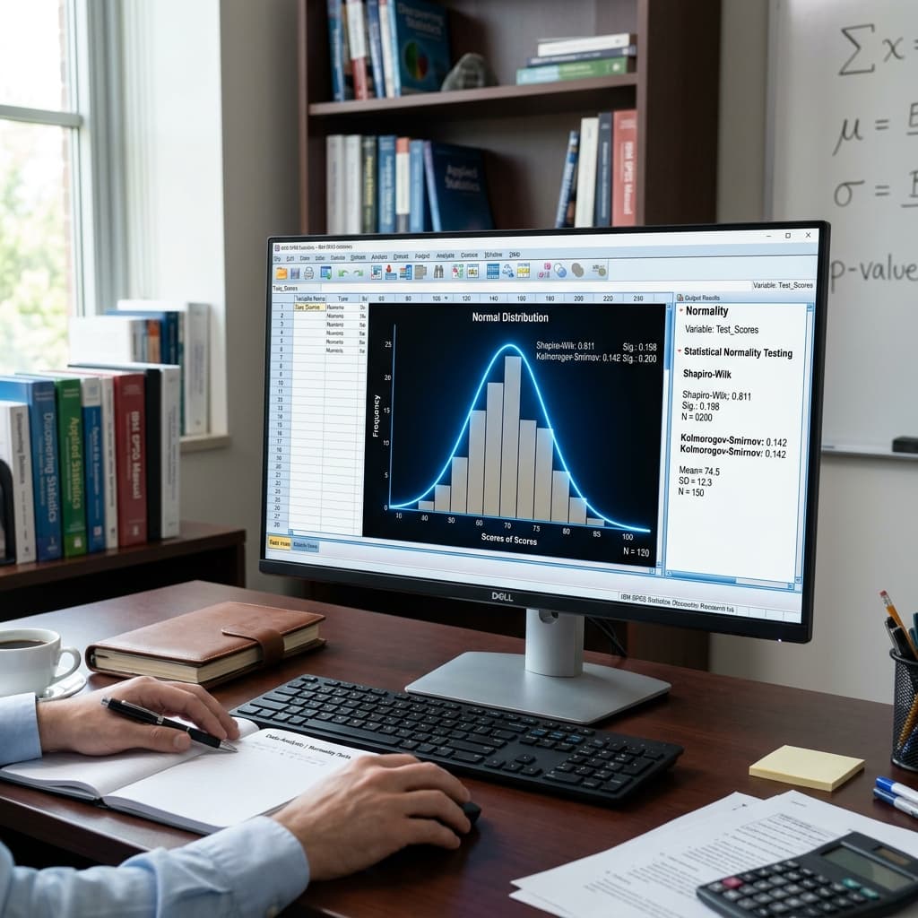
Before you can dive into the results of a one-way ANOVA or interpret a Pearson correlation, you face a crucial decision gate: the assumption of normality. Almost every introductory statistics course hammers home the idea that parametric tests require normally distributed data. But what does that actually mean in practice? And more importantly, how do you correctly assess normality using IBM SPSS Statistics without falling into common interpretative traps?

In this comprehensive guide, we will unpack the concept of statistical normality, explore the various graphical and numerical methods for assessing it in SPSS, and clarify several pervasive misconceptions about what statistical tests for normality actually tell you. By the end of this article, you will not only know which buttons to click in SPSS, but you will also understand the nuanced interpretation required to make sound methodological decisions. If you are ever in doubt about which test to use after assessing your data, our Statistical Test Decision Tree is a handy reference.

Understanding the Concept of Normality

The normal distribution, often visualized as a symmetrical "bell curve," is a foundational concept in inferential statistics. In a perfectly normal distribution, the mean, median, and mode are all equal and located at the exact center of the distribution. The spread of the data is dictated by the standard deviation, following the empirical rule (approximately 68% of data falls within one standard deviation of the mean, 95% within two, and 99.7% within three).

Why do we care? Many popular inferential statistical procedures—collectively known as parametric tests—are mathematically derived based on the assumption that the sampling distribution of the mean is normally distributed. While the Central Limit Theorem states that the sampling distribution of the mean approaches normality as the sample size increases (regardless of the underlying population distribution), smaller sample sizes require the population distribution itself to be approximately normal for these tests to maintain their stated Type I error rates and statistical power.

However, a critical nuance often lost is that parametric tests do not always assume that the raw data itself is normally distributed. For instance, in linear regression, the assumption of normality applies to the residuals (the errors), not the independent or dependent variables themselves. Always verify exactly what needs to be normal for your specific test.

Visualizing Data: Graphical Methods for Assessing Normality

Before looking at p-values from statistical tests, your first step should always be to visualize your data. Graphical methods provide an intuitive understanding of your data's shape, spread, and potential outliers. While subjective, they are less prone to the sample size sensitivities that plague formal statistical tests.

1. Histograms

A histogram groups continuous data into "bins" and displays the frequency of observations within each bin as a bar. Overlaying a normal curve on a histogram in SPSS allows for a quick visual comparison between your empirical data and an idealized normal distribution.

How to create a histogram with a normal curve in SPSS:

• Go to Graphs > Chart Builder...
• In the Gallery tab, select Histogram.
• Drag the simple histogram icon into the preview canvas.
• Drag your continuous variable onto the X-Axis.
• In the Element Properties window on the right, check the box for Display normal curve.
• Click OK.

Interpretation: Look for symmetry around the center. Are the tails roughly equal in length? Is there a single, central peak? Be cautious: histograms can look drastically different depending on the number of bins chosen by the software. They are a good starting point but rarely definitive on their own.

2. Normal Q-Q Plots (Quantile-Quantile Plots)

A Q-Q plot is arguably the most reliable visual tool for assessing normality. It plots the quantiles of your observed data against the expected quantiles of a theoretical normal distribution. If your data is perfectly normal, the points will fall exactly along a 45-degree reference line.

How to generate a Q-Q Plot in SPSS:

• Go to Analyze > Descriptive Statistics > Q-Q Plots...
• Move your variable into the Variables box.
• Ensure the Test Distribution is set to Normal.
• Click OK.

Interpretation: Deviations from the line indicate departures from normality.

• If the points curve upwards at both ends (like a smile), the distribution is skewed to the right (positive skew).
• If the points curve downwards at both ends (like a frown), it is skewed to the left (negative skew).
• An S-shape indicates issues with kurtosis (heavy or light tails).

Minor deviations, especially at the extreme tails, are common in real-world data and often acceptable.

Numerical Methods: Skewness and Kurtosis

Beyond visual inspection, calculating descriptive statistics quantifying the shape of the distribution provides a more objective measure of normality.

Skewness

Skewness measures the asymmetry of the distribution.

• A skewness value of exactly 0 indicates perfect symmetry (a perfectly normal distribution).
• A positive value indicates positive skewness (a long tail stretching to the right, towards higher values).
• A negative value indicates negative skewness (a long tail stretching to the left, towards lower values).

Kurtosis

Kurtosis measures the "tailedness" of the distribution—how much data is in the tails compared to the center. It does not measure "peakedness," which is a common misconception.

• Mesokurtic (Kurtosis = 0 in SPSS): The distribution has tails similar to a normal distribution. (Note: SPSS calculates excess kurtosis, where 0 is normal).
• Leptokurtic (Positive Kurtosis): The distribution has heavier, fatter tails than a normal distribution (more extreme outliers).
• Platykurtic (Negative Kurtosis): The distribution has lighter, thinner tails than a normal distribution (fewer extreme outliers).

Rule of Thumb: While strict cut-offs vary, a common guideline suggests that skewness and kurtosis values between -1.0 and +1.0 (or sometimes -2.0 and +2.0) are considered acceptable to prove an approximately normal distribution for many parametric tests. However, dividing the skewness or kurtosis value by its standard error to get a z-score (e.g., Z_skewness = Skewness / Standard Error of Skewness) is a more rigorous approach. If the resulting z-score is outside the range of -1.96 to +1.96, the departure from normality is statistically significant at the p < .05 level.

Formal Statistical Tests for Normality

SPSS provides formal null hypothesis significance testing (NHST) for normality. The null hypothesis (H₀) for these tests is that the data is normally distributed. The alternative hypothesis (H₁) is that the data is not normally distributed.

The Shapiro-Wilk Test

The Shapiro-Wilk test is generally considered the most powerful test for normality, especially for smaller sample sizes (N < 50), although it performs well up to N = 2000. It compares your data's variance to a theoretical variance calculated from a normal distribution.

The Kolmogorov-Smirnov (K-S) Test

SPSS also outputs the K-S test (specifically the Lilliefors corrected version). It compares the cumulative distribution function of your data to that of a normal distribution. Generally, statisticians recommend prioritizing the Shapiro-Wilk test over the K-S test due to higher power.

How to run these tests in SPSS:

• Go to Analyze > Descriptive Statistics > Explore...
• Move your continuous variable to the Dependent List.
• Click on the Plots... button.
• Check the box for Normality plots with tests.
• Click Continue, then OK.

In the output, locate the "Tests of Normality" table. Look at the "Sig." (p-value) column for the Shapiro-Wilk test.

• If p < .05, you reject the null hypothesis. The data significantly deviates from a normal distribution.
• If p > .05, you fail to reject the null hypothesis. There is not enough evidence to say the data is non-normal.

CRITICAL WARNING: The Trap of Statistical Tests

Many researchers blindly rely on the Shapiro-Wilk test to make their decisions, which is a dangerous practice. We must explicitly state two crucial statistical truths that are frequently misunderstood:

The Synthesis: How to Actually Make a Decision

Because visual methods are subjective and statistical tests are fatally sensitive to sample size, assessing normality is not a binary "yes/no" checkbox. It is a holistic judgment call. Here is a recommended workflow:

1. Always start with visuals. Look at the Q-Q plot and the histogram. Does it look roughly bell-shaped? Are the deviations on the Q-Q plot minor or severe? Are there massive outliers distorting the picture?
2. Check Skewness and Kurtosis. Are the values within an acceptable range (e.g., -1 to +1)? This provides a quantitative backing to your visual assessment that isn't solely dependent on a p-value.
3. Consider the Sample Size.
   • Small Sample (N < 30): You must be cautious. Visuals are hard to interpret. If Shapiro-Wilk is significant, you should strongly consider non-parametric alternatives, as parametric tests are not robust here.
   • Medium Sample (30 < N < 100): Use a combination of visuals, skew/kurtosis, and the Shapiro-Wilk test. Minor violations are likely fine.
   • Large Sample (N > 100): Ignore the Shapiro-Wilk test entirely; it will almost certainly be significant due to power. Rely solely on visual inspection (Q-Q plots) and skewness/kurtosis values to ensure the deviation isn't wildly extreme. The Central Limit Theorem protects your parametric tests here.
4. Consider the specific statistical test. Some tests are more robust than others. For example, a two-sample t-test with equal group sizes is highly robust to non-normality.

What to Do if Your Data is Severely Non-Normal

If you conclude that your data is too severely skewed or kurtotic to justify a parametric test, you have several options:

• Data Transformations: You can apply mathematical transformations (e.g., logarithmic, square root, inverse) to pull outliers in and normalize the distribution. Note that this changes the interpretation of your variables.
• Non-parametric Tests: You can use alternative tests that do not assume normality (e.g., Mann-Whitney U instead of an independent t-test, Kruskal-Wallis instead of a one-way ANOVA, Spearman's rank correlation instead of Pearson correlation).
• Robust Statistical Methods: Modern approaches like bootstrapping do not rely on strict distributional assumptions and can provide robust standard errors and confidence intervals.

---

Frequently Asked Questions (FAQ)